|
I have a lot of duplicates in the reports that I run and often need to quickly identify them to see if my lists match or if I need to remove them so I don’t have duplicate information.  Luckily, Excel makes this process very easy! First, we’ll check our data for duplicates. 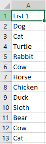 From the list above, we can see that I have a few animals listed more than once. To identify them, we will use Conditional Formatting. First, highlight the area that you want to apply conditional formatting. You can select a series of cells, rows, columns, or the entire sheet. Once you have your data selected, you will go to the Home tab of your ribbon. In the middle, there is a drop down called “Conditional Formatting.” 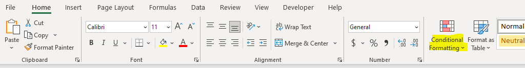 Click on “Conditional Formatting” to open the drop down. Select Highlight Cells Rules and then Duplicate Values.  You will get a popup that will give you a preview of what will be formatted. The default is Light Red Fill with Dark Red Text, but you can select other colors or you can select Custom Format to choose the formatting that will help you identify the duplicates. Click OK. 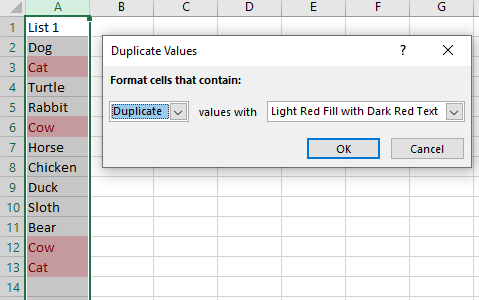 Now I can see that I have two Cats and two Cows listed. If I had three, it would still work. This is great because I can see that I did have duplicates in my list, but now I want to delete them. If I have a large set of data, it may take me a while to delete each one, so we are going to use the built-in “Remove Duplicates” tool within Excel. On the Data tab of your ribbon under the Data Tools section, you will find a button called “Remove Duplicates.” 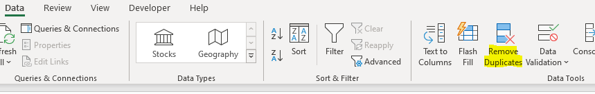 You just need to highlight the data that you’d like to apply the removal to and click the “Remove Duplicates” button. 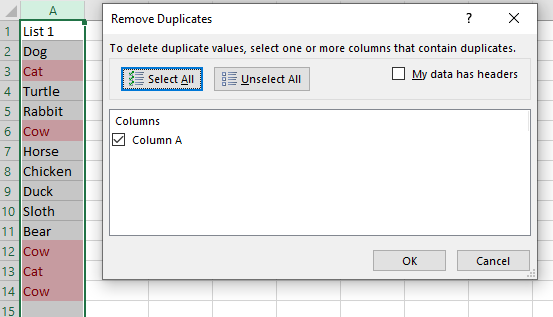 If you have headers, you can check the “My data has headers” box in the upper right. This will change the names of the available columns to match your headers instead of saying “Column A” mine would say “List 1.” If you have multiple columns, say the animals in A and the price in B and the data in B is not the same, you can uncheck Column B. It will only look for duplicates that exist in Column A and will delete the entire row if it finds a duplicate. This can be very helpful, just know that it will keep the top most item and delete the duplicates that are farther down the list. Make sure that you have your data sorted in the appropriate order so that the records you want to keep are at the top before deleting the duplicates. 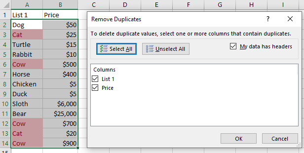 For my example, I’m going to uncheck the “Price” because I know my current prices are at the top of the list and I still want to remove the duplicate animals. 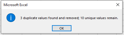 Once you hit OK, you will get a popup that confirms how many duplicates were removed and how many unique values remain. This will also tell you if there were no duplicates found so you can just use it to confirm that there are none. 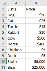 You can see that my $25 Cat and $500 Cow remained on the list while the others were removed and the other rows moved up so there are no blank rows. Both of these methods are great to use and you can go straight to the “Remove Duplicates” if you know you want to delete them or want to confirm you don’t have any. Sometimes, you don’t need to remove the duplicates, but need to identify them to confirm that your lists are the same (or not the same). I use this method a lot if I’m updating a style list or something where I need to make sure that I’ve captured all of the items that I was intending to. If you paste your lists next to each other, you can apply conditional formatting to find the duplicates and highlight the cells that are the same. I would advise you to remove duplicates ONE COLUMN AT A TIME first. If you apply the conditional formatting and you have a duplicate in the same column, it will highlight it as a duplicate which may be misleading if you’re trying to see duplicates from one column to the other. Here’s the data I’m going to start with. I have List 1 and List 2. I can see that List 2 is missing an animal because it’s shorter, but instead of re-sorting and manually hunting for it (and straining my eyes beyond belief) I will use the conditional formatting. 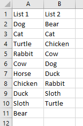 I’m going to start by highlighting columns A and B. Then go to Home>Conditional Formatting>Highlight Cells Rules>Duplicate Values. For this one, I want to get a little fancy, so I’m going to select Custom Format. I get another popup that has multiple text formatting options. I’m going to select “Bold Italic” under Font Style and choose pink on the Fill tab. 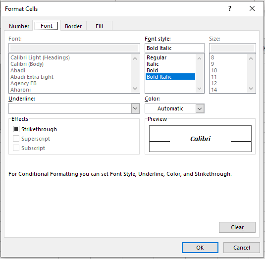 This gave me a very different visual than the first example, but I can clearly see that Horse is the animal that I’m missing from List 2. 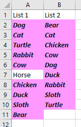 If you need to do any data validation, this tool is crucial. Conditional Formatting has so many options and I will continue to write guides on them. If there’s one that you’re interested in seeing, let me know in the comments below! If you have any issues or questions, please reach out by sending an email!
0 Comments
Leave a Reply. |
|||
